CE.adsp: Laboratory 1

You're not expected be able to finish all the laboratory exercises in the time available, so just try to get as much out of it as you can. Please ask one of us if you get stuck on anything.

If you've got this far, then you'll have already logged in and opened a browser. The lab uses the signal processing capabilities of Matlab, which is a popular numerical analysis package, and comprises three main components:

1. Fundamentals: generating some simple waveforms and their spectra, basic filtering;
2. Speech processing: two methods of pitch analysis, extraction of spectral characteristics;
3. Advanced exercises: Wiener filter, Hartley transform and adaptive line enhancement.

Getting started

Before you begin your Matlab session, you'll want to create a directory in your home directory where you can store any programs and data that you use. At the command prompt (i.e., in a terminal window), type "mkdir matlab" which you can see listed with the ls command in Linux/Unix. You can enter this directory as in DOS, with "cd matlab". To start Matlab, type "matlab &" at the prompt (& will leave the command window active). Once Matlab has fired up, there are a number of resources available to you:

• "helpwin" opens the help window;
• "helpdesk" calls up the Matlab documentation on the Mathworks website (as does "?");
• "edit" allows you to view and edit a program;
• "demo" opens the help on demonstrations.

Scripts and functions can be edited either in the Matlab editor or using a standard text editor. For example, to edit a file called sigdemo1.m, simply type "edit sigdemo1" in the Matlab command window, or you could use gedit from within your original terminal window: "gedit yourfile.m &".

To run a script (a .m file containing a list of instructions), just enter the filename without its extension into the Matlab command window: e.g., "sigdemo1".

1. Fundamentals

If you are new to Matlab, click on the Help menu (see toolbar) and then click on "Demos", that is, [Help | Demos]. This will give you an idea to some of Matlab's capabilities. If you have some experience with the signal processing toolbox, proceed to section 2; experts, please go on to section 3 or invent your own variations of the parts that interest you most.

1.1 Demonstrations

Type "sigdemo1" at the Matlab command prompt, and investigate the spectra produced by some common signals. This demonstration also allows you to see the effects of different window functions on the resultant spectra.

Type "phone" at the prompt to see an example of a simple coder.

1.2 Generate a sine wave

There are (at least!) two ways to work in Matlab. The first, and simplest, involves entering commands directly at the command prompt. Let's begin by setting the sample rate to 100 Hz: "Fs = 100". Matlab will respond with the variable Fs and echo its value of 100. To suppress this response, which can become annoying with vectors and matrices of data, put a semicolon at the end of the line.

Next, define a time vector with which to sample the waveform, running from 0 s to 1 s in steps of 1/Fs:

t = (0:1/Fs:1)';

The second way of programming in Matlab is to create a text file using the editor. By listing commands in a script file, we can get Matlab to execute them as if they were entered at the command prompt. Type "edit" and then enter the following text (you can ignore anything after "%", which indicates a comment):

Fs = 100;	% sampling frequency (100Hz)
t = (0:1/Fs:1)';	% initialise time vector
y = 2*sin(2*pi*10*t);	% A sin(wt)
plot(t,y);	% plot t against y

1.3 Display the spectrum

Add the following lines of code to your text file, and run it to display the spectrum of the sine wave:

Y = fft(y);
f = (0:length(Y)-1)*Fs/length(Y);	% initialise frequency vector
magnitude = abs(Y);
phase = unwrap(angle(Y));
figure(2)	% open a new figure window to keep the first
plot(f,magnitude);
figure(3)
plot(f,phase*180/pi);

1.4 Using a square wave

Repeat the previous two exercises using a square wave, instead of a sinusoid. Use the help window to find the command (if you can't guess it!).

1.5 Low-pass filtering

Use the commands "fir1", "freqz" and "filter" to design a low-pass filter that will convert the square wave back into a sine wave. Think carefully about the filter order and its cut-off frequency. Note that Matlab uses normalised frequencies in its filter specifications, so the cut-off frequency must be divided by the Nyquist frequency (viz., half the sampling frequency).

Examine the effects of varying these parameters, the order and cut-off frequency.

Try, and investigate the differences, of using different window functions in "fir1", such as boxcar (rectangular), bartlett (triangular), hamming, blackman, etc.

2. Speech processing

This section applies some signal processing techniques to a speech waveform. An example file can be saved by right-clicking over the following link: speech.wav. You can load the contents of this file into Matlab using wavread (conversely, you can save a waveform to file with wavwrite):

[y,Fs] = wavread('speech.wav');

Voiced speech is strongly periodic, since tension of the vocal cords is adjusted by the larynx so that they vibrate in a fairly regular fashion. During unvoiced speech, the lungs force air through constrictions within the vocal tract which produce turbulence. An example is the /s/ sound (fricative) at the beginning of the word "speech".

2.1 Pitch period from time domain

Find a section of voiced speech in your waveform, and copy it to a smaller array. Observe the pitch pulses and estimate the pitch period of the voiced speech from the waveform. The pitch period in human speech typically lies in the range 4-20 ms.

2.2 Formants from spectral envelope

Examine the spectrum of the 30 ms window of speech and estimate the formant frequencies. First draw an imaginary line joining the peaks of the spectrum to form a spectral envelope. Then look for humps in this envelope and estimate their centre frequencies. These are known as the formant frequencies. Formants are caused by resonances in the vocal tract, and there should be about five of them in the first 5 kHz.

2.3 Pitch period from autocorrelation

Low-pass filter the voiced speech, with a cut-off frequency of 800 Hz, the examine the results of the autocorrelation function xcorr, with maxlags set to 100. Observe the maximum correlation after the zeroth lag (remember that the zeroth lag corresponds to 100, in this case, since the autocorrelation function is symmetrical about maxlags).

Re-estimate the pitch period from the autocorrelation function, and compare it to the one you obtained from the time waveform.

2.4 Linear predictive analysis

Now, find the spectral envelope using linear prediction (see lpc), and compare it to the original spectrum. Think about the order of your filter and see the effect of varying it.

The following commands may help you, where a is a vector of LPC coefficients:

impulse = [1; zeros(N,1)];	% generate a Kronecker delta impulse for N >1
synthesis = filter(1,a,impulse);	% impulse response for all-pole model (synthesis filter)
analysis = filter(a,1,impulse);	% impulse response for all-pole model (analysis filter)

Reconstructing the frame of speech (synthesis) is achieved by passing the residual through an all-pole model (synthesis filter), which is simply the inverse of the analysis filter.

2.5 Real cepstrum

1. Implement the real cepstrum:

   c_s(ν) = F ^-1{ln|F{s(n)}|},

   where F denotes the discrete Fourier transform (DFT) and ν is discrete quefrency (i.e., sampled).
2. Perform cepstral deconvolution (homomorphic decomposition) on the same section of speech as used in section 2.4, and compare the resulting spectral envelope to that from linear prediction.
3. Calculate the pitch period and compare your results to linear prediction. from linear prediction.

3. Advanced exercises

3.1 FIR Wiener filter

Using the block diagram shown in Figure 1, design a 40th-order Wiener filter for the aplpication of noise cancellation (see also section 3.3, below), where

W = R^-1p

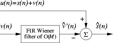
Figure 1. Mth-order FIR Wiener filter.

3.2 Hartley transform

1. Implement the Hartley transform (Hint: use "fft").
2. Generate a short pulse-like signal of 100 samples, with 10 ones (pulse) and 90 zeros:

   pulse-signal = [ones(10,1); zeros(90,1)];

3. Calculate the magnitude spectrum and phase spectrum of this signal.
4. Now shift the pulse in time and examine the change in phase.
5. Repeat steps 3 and 4 nutil the pulse has been shifted to the end of the vector.

3.3 Adaptive line enhancement

Adaptive line enhancement (ALE) refers to the case where a noisy signal u(n), consisting of one or more sinusoidal components s(n), is available and the requirement is to remove the noise part of the signal v(n). This may be achieved by the arrangement of Figure 2, below. It consists of a de-correlation stage, symbolised by z^-Δ and an adaptive predictor. The decorrelation stage attempts to remove any correlation that may exist between the samples of noise, by shifting them Δ samples apart. As a result, the predictor can only make a prediction about the sinusoidal components of u(n), and when adapted to minimise the output mean-squared error (MSE), the line enhancer will be a filter tuned to those sinusoidal components.

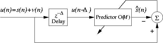
Figure 2. Mth-order adaptive line enhancer.

See if you can use the LMS algorithm to control a 40th-order FIR filter to enhance a 100 Hz sine wave corrupted by noise. You might find it informative to plot the frequency response of the filter at each iteration, and then finally display the output plotted over the input, for comparison.

1. Adjust the amplitude of the noise source and the frequency of the sine wave;
2. Modify the value of μ used in the update, and see what happens. At what value of μ does the algorithm become unstable?

• Mathworks
• Matlab central
• Matlab FAQ
• Matlab product details
• Local help
• UniS users' group

If you have any other specific questions outside of the lab, you can email me, and I'll do my best to respond swiftly.