EEM.ssr: Lab 3 - HMM decoding and training

Assessment:	students should work individually and submit their results in the form of a short technical report as a PDF file via SurreyLearn to Dr Jackson before 4pm on Tuesday 13 May 2014
Required software:	Matlab (v.7) is the recommended application for this laboratory
Additional software:	HTK (v.3.4.1) for feature extraction, Excel for spreadsheet calculations

Aims of the Experiment

To gain experience of HMM decoding and training using features extracted from your recorded speech signals by HTK. To deepen your understanding of the Viterbi and Expectation-Maximization algorithms through Matlab implementation and experimentation.

Recommended reading

• Young et al.: Young, S.J. et al., The HTK Book, CUED (v3.4), 2006. website | pdf (on campus only)
• Rabiner: Rabiner, L.R., A tutorial on HMM and selected applications in speech recognition, In Proc. IEEE, Vol. 77, No. 2, pp. 257-286, Feb. 1989.

1. Preparation

In preparation for the lab, you should:

• Make sure you have the HTK-MFCC files that you created in the previous practical.
• Understand how to calculate the probability density for a multivariate Gaussian distribution.
• Familiarise yourself with the Baum-Welch equations for re-estimating HMM parameters.
• Identify any Matlab functions you may need, such as: max, log and diary.

Here are some useful functions, examples and resources that you can find in the lab3 directory:

• MultiGauss.m, LogMultiGauss.m - Matlab functions for computing multivariate Gaussian proabilities and log probabilities
• LogAddProb.m - Matlab functions for computing the sum of two log probabilities, for use in the forward and backward procedures
• assignment_SURNAME.tex, assignment_refs.bib, assignment_SURNAME.pdf - a LaTeX document template that can be used for writing the assignment report

2. Overview

An overview of the tasks for this assignment is as follows:

1. Using the MFCC features previously extracted with HTK from your speech recordings and a prototype HMM from last time, run the Viterbi algorithm to get the best path and its cumulative likelihood.
2. Calculate the likelihoods required for Baum-Welch training.
3. Perform model re-estimation and re-evaluate the best path.
4. Present the results in the form of a brief technical report.

The deliverable to be submitted is a short technical report that should contain the following results:

1. Running the Viterbi algorithm:
   1. the observation likelihoods for each state in your model λ_three with your utterance "three"
   2. the best path X* when using the corresponding model λ_three
   3. its cumulative likelihood Δ* = p(O,X*|λ_three)
   4. best path and cumulative likelihood using a different model λ_oh on the same observations
2. Calculating likelihoods for Baum-Welch training:
   5. the forward likelihoods α_t(i) and observation likelihood p(O|λ_three)
   6. the backward likelihoods β_t(i)
   7. the occupation likelihoods γ_t(i)
   8. the transition likelihoods ξ_t(i,j)
3. Re-estimating the model and evaluating the new best path:
   9. re-estimated model parameters λ′_three = {A′, B′} where B′ = {b′_i} for i=1..5 and b′_i = {μ′_i, Σ′_i}
   10. best path and cumulative likelihood using the updated model λ′_three
4. Presenting the results in a technical report:
   • Title page -- assignment title "HMM decoding and training report", your name, module code (EEEM034), my name (Dr Philip Jackson), date
   • Abstract -- an executive summary of the contents of the report
   • Glossary -- an optional list of symbols and their meanings
   • Introduction -- a brief description of the assignment
   • Method -- a statement of the equations used to calculate the results and any important implementation details
   • Results -- a complete set of the results for each point, typically in tables
   • Conclusion -- a summary of what you did, statement of the main findings and a short discussion of any points of interest
   • References -- a list of any relevant texts that are cited in standard IEEE format
   • Appendix -- you can include any intermediate results or evidence of your working here, along with program listings for any code that you have authored

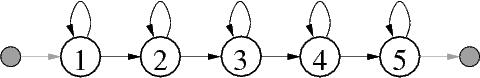Figure 1: HMM state topology for the prototype, including entry and exit null states.

3. Experimental Work

3.1 Running the Viterbi algorithm

1. Extract the observation sequence O from your utterance "three" by taking the whole of the middle section that corresponds to the spoken word. Given your initial values of μ_i and Σ_i in your initial model for this word λ_three, calculate the output probability b_i(o_t) on these observations O={o_t} at every time t={1..T}. Note that the values will be identical for emitting states 1, 2, 3, 4 and 5, since you have used the same mean and diagonal covariance in each state.
2. By implementing the Viterbi algorithm in Matlab, find the best path X* for these observations using the initial parameters λ_three = {A, B} where A = {a_ij} for i,j=1..5, and B = {b_i} for i=1..5 and b_i = {μ_i, Σ_i}.
3. Report the cumulative likelihood Δ* = p(O,X*|λ_three) along that path.
4. Repeat the above three steps using the initial model representing the word "oh", and report the best path and cumulative likelihood with that model λ_oh.

3.2 Calculating likelihoods for Baum-Welch training

5. Using your initial parameters λ_three, compute the forward likelihoods α_t(i) throughout the trellis, i=1..5 and t=1..T, and record the observation likelihood p(O|λ_three).
6. Taking β_t(i) for i=1..5 based on the exit probabilities η_i, calculate the backward likelihoods β_t(i) throughout the trellis, t=1..T.
7. Using your values of α_t and β_t from the previous steps, compute the occupancy likelihoods γ_t(i) for each node in the trellis, t=1..T.
8. Also using α_t and β_t, calculate the transition likelihoods ξ_t(i,j) for each connection within the trellis between states i and j, t=2..T.

3.3 Re-estimating the model and evaluating the new best path

9. Use the values of γ_t and ξ_t from the previous section to re-estimate the parameters of the model, λ′_three = {A′, B′}, according to the Baum-Welch formulae, where B′ = {b′_i} and b′_i = {μ′_i, Σ′_i} for i=1..5.
10. Finally, re-compute the best path X* and cumulative likelihood p(O,X*|λ′_three) using the updated model λ′_three.

3.4 Assignment submission

1. Collate the results identified as deliverables in section 2 within one file as a short technical report, using tables and appendices as appropriate.
2. Produce a PDF version of the document, e.g., called lab3_YourName.pdf.
3. Submit the file as assignment 3 in SurreyLearn.

4. Further work

It is beyond the scope of this assignment to train all the models and to perform recognition tests of every word with every model. However, having written the programs to do this already, you may be interested to see whether your digit recognizer works. Good luck!

FAQ. Questions and answers

Here are some questions from students together with my answers that you may find helpful in completing the assignment.

Q.1

I'm not certain on how the HMM relates to the MFCC relates to the trellis diagrams you used in the lectures etc.

A.1

The MFCCs represent the observations (as a sampled continuous 39-D vector sequence). The HMM is a model that acts as the template. In the trellis diagram the observation sequence goes along the x axis, and the states of the HMM up the y axis.

Q.2

So the MFCCs define the sequence of output emission probabilities for each state, b_i(o_t) which is a scalar calculated from the 39-D multivariate gaussian equation. Then for each time step on the x axis, there are 5 corresponding emission probabilities (one for each state). But in the initial model these are all the same. How does that affect the path? Also, I've used π=[1 0 0 0 0], η=[0 0 0 0 1]^T and A = [0.4 0.6 0 0 0; 0 0.4 0.6 0 0; 0 0 0.4 0.6 0 ... etc.]. Were there any constraints on these because they obviously affect the model? Aren't the observations duplicated for each state?

A.2

Yes, you're right. The observations can be used with any state. The only constraints are at the start and the end where the path must pass through the first and the last states respectively. Your implementation of the Viterbi algorithm will determine the actual path that's output as the best one (because there are paths that have identical probability). Note that the self-loop and onward transition probs are the other way round in the prototype, 0.6 and 0.4 respectively; the exit prob has a value of η=0.4 for the final emitting state.

Q.3

With regards to the SSR coursework, when we're attempting to calculate the output probability of the observations using MultiGauss.m, I'm a little confused as to what the vector of observation points is. I have tried using a 39x1 vector, a 39x39 matrix of zeros, ones etc. but I keep getting the error in the end of: Matrix is close to singular or badly scaled and the output probabilities are all zero-valued. Could you perhaps clarify what this vector is and how large it is expected to be?

A.3

At each time step, the observation vector is a 39x1 feature vector taken from the MFCC file and corresponding to the current time frame. The mean is also a 39x1 vector and is taken from the prototype model that you produced. The covariance matrix should be a diagonal matrix with the elements of variance from the model along the diagonal and zeros elsewhere. With these parameters, the MultiGauss function ought to give non-zero values most of the time. However, when working with linear probability values, underflow is a problem that occurs frequently (even in Matlab!), so you may want to consider converting your program to the log prob version. Nevertheless, it is useful to have both as it allows you to verify the first few frames of your implementation against hand calculations in both cases.

Q.4

Are the probabilities for the forward and backward procedures over this size trellis still going to come out to be identical? Mine are different!

A.4

Yes, they should do (to within the precision of the application). Are you sure you've not missed out a term in the calculation of one of them?

[ Home | Section: 1, 2, 3, 4, FAQ | Dr Jackson ] © 2010-14, written by Philip Jackson, who maintains it, last updated on 21 March 2014.